4.6. Visualization export
In addition to CityGML and CityJSON, 3D city model content stored in a 3D City Database can also be exported as KML [Wils2008], COLLADA [BaFi2008], and glTF [Khro2018] on the VIS Export tab shown below for visualization and use in a broad range of applications such as Earth browsers like Google Earth, ArcGIS Explorer, and Cesium.
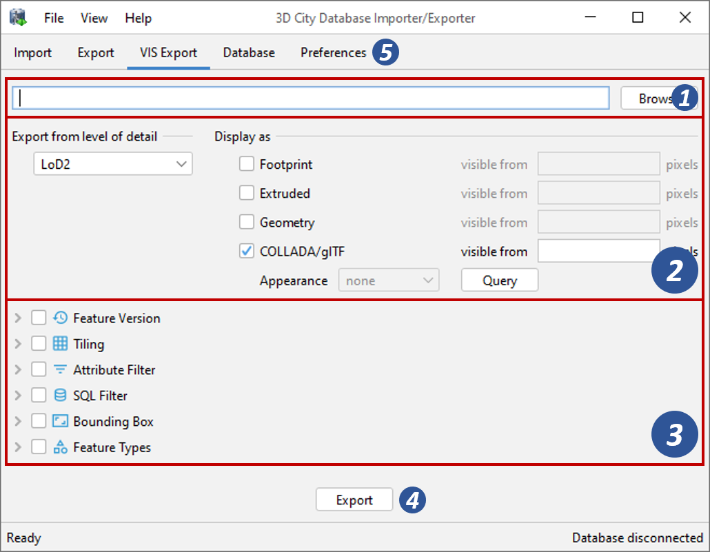
Fig. 4.73 The VIS Export tab allowing for exporting visualization models from the 3DCityDB.
On the VIS Export tab, all parameters required for the export have to be entered in a similar fashion like for a CityGML/CityJSON export (see Section 4.5). Mandatory input is the output file [1], the Level of Detail (LoD) to export from as well as the display forms [2].
Output file selection
The path and filename of the main output file must be provided at the top of the dialog [1]. You can either manually enter the output file or use the Browse button to open a file selection dialog. This output file is always created as KML file that uses the KML network link mechanism to link the separate datasets containing the visualization models that are created during the export process. For most viewers and applications (e.g., Google Earth) it should be sufficient to just load this main output file. The viewer can parse and follow the links in this file to conditionally load and refresh the visualization models.
Since the format of the main output file is always KML, it is recommended to use
.kml as file extension.
Level of Detail to export from
The export dialog lets you choose the LoD representation of the city objects that shall be used for creating the visualization models [2]. The corresponding drop-down list offers the five levels LoD0 - LoD4 as defined by CityGML and “highest LoD available” as additional option (default: LoD2).
For each top-level city object, the export operation will only query the geometry in the selected LoD and use this geometry as basis for the visualization export. Also child objects such as boundary surfaces of buildings are searched for geometries. If a geometry can neither be found for the top-level city object nor one of its child objects in the given LoD, the object will not be exported.
When choosing “highest LoD available” rather than a specific LoD, the process will iterate from LoD4 to LoD0 for every city object and search for a geometry representation according to the above scheme. The first geometry found will be used for the visualization export. This way, every city object will be included in the export data, unless it has no geometry at all.
Note
The geometry representation of city objects usually gets more detailed and complex with higher LoDs. Thus, the visualization gets more detailed as well, but the export may take longer to generate the models. Likewise, file sizes increase and loading the models in Earth browsers might be slower. Tiled exports help to keep the file sizes small and loading times fast.
Display forms
Besides the LoD, also the way the models shall be displayed (display form) must be specified [2]. The user can choose one or more display forms. Each display form is generated based on the geometry of the city object in the specified LoD and also determines the output format of the corresponding visualization models. The following display forms are available:
Display form
|
What is visualized
|
Output format
|
Footprint
|
Objects are represented by a ground surface that is derived by projecting its geometry onto the earth surface.
|
KML
|
Extruded
|
Objects are represented as block models by extruding the Footprint representation to the highest point taken from the 3D bounding box.
|
KML
|
Geometry
|
Objects are represented with their full geometry.
|
KML
|
COLLADA/glTF
|
Objects are represented with their full geometry. In contrast to Geometry, this display form also supports textures.
|
COLLADA and/or glTF
|
Note
The display forms Extruded, Geometry and COLLADA/glTF are not only available when exporting from LoD0.
By default, all visualization models created from the exported city objects are organized into one visualization dataset per display form. Alternatively, you can choose to apply tiling (see below) which will result in one dataset per tile and display form. The datasets will contain the name of the display form as suffix in the filename, so that they can be easily identified and kept apart.
The following figure exemplifies the different display forms for one building. All representations have been derived from the LoD2 representation of the building.
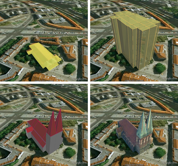
Fig. 4.74 The same building displayed as Footprint, Extruded, Geometry, COLLADA/glTF with textures (from top left to bottom right)
If you want to create a visualization with textures or colors stored as appearances in the 3DCityDB, select the COLLADA/glTF display form and additionally pick an appearance theme from the drop-down list in [2] (default: none). Click the Query button to populate this drop-down list with the themes available in the database. If you have not established a database connection beforehand, the Importer/Exporter will automatically connect to the currently selected database entry on the Database tab to retrieve the list of appearance themes.
With the visible from input field next to each display form [2], you can control the visibility of the visualization models created for the separate display forms. When the contents of a dataset are projected onto the screen in the viewer, they must occupy an area of the screen that is greater than the number of pixels specified in visible from (in square pixels) in order to become visible. When exporting more than one display form at the same time, the visible from value of a higher-resolution display form also defines when a lower-resolution display form shall become invisible. This enables to seamlessly switch between the different display forms in a viewer when zooming in and out.
For example, assume you export your city objects as Extruded with visible from set to 50 and as Geometry with visible from set to 200. If you open the scene in a viewer and zoom into it, then the extruded models will first occupy an area of 50 pixels and thus will become visible. When you zoom in more and the screen space criteria is fulfilled for the Geometry dataset, the Geometry dataset will become visible and the Extruded models are not displayed any more. When you zoom out again, the viewer will switch back to the Extruded display.
Note
In the main KML output file, the visible from input values are mapped onto
<minLodPixels> and <maxLodPixels> properties of different
<Region> elements, with each <Region> representing
one visualization dataset (also see [Wils2008]). The last display
form in the list receives a value of -1 for <maxLodPixels> and, thus,
will not become invisible when zooming in even more. A viewer must support these
KML elements in order for the switching between display forms to work.
Note
Proper values for the visible from values depend on both the spatial extent and the file size of a visualization dataset. Thus, the values must always be adapted to a specific export. An example for a good combination for typical LoD2 city objects and a tile size of 250x250m could be:
- Footprint visible from 50 pixels,
- Extruded visible from 125 pixels,
- Geometry or COLLADA/glTF visible from 200 pixels.
Caution
For Oracle, the Footprint and Extruded display forms are implemented based on the spatial function SDO_AGGR_UNION. This function is not included in Oracle 10g/11g Locator but requires Spatial for these database versions. Starting from Oracle 12c, the function is also included in Locator.
Export filters
The visualization export operation offers thematic and spatial filters to restrict an export to a subset of the 3D city model content stored in the database [3]. The following filters are available and discussed in separate sections of this chapter:
- 4.6.1 Feature version filter
- 4.6.2 Tiling filter
- 4.6.3 Attribute filter
- 4.6.4 SQL filter
- 4.6.5 Bounding box filter
- 4.6.6 Feature type filter
To enable a filter, simply select its checkbox. This will automatically make the filter dialog visible. Make sure to provide the mandatory input for the filter to work correctly. If more than one filter is enabled, the filters are combined in a logical AND operation, i.e. all filter criteria must be fulfilled for a city object to be exported. If no checkbox is enabled, no filters are applied and, thus, all features contained in the database will be exported.
Note
All export filters are only applied to top-level features but not to nested sub-features.
Tiled exports
When exporting 3D city model content to a single visualization file, the file size may quickly grow. The performance of a viewer application may significantly drop for large files if the data can be displayed at all, especially when using a web client for visualization. It is therefore strongly recommended to use tiling for visualization exports. With tiling enabled, the area to be exported is split into a regular grid of tiles, and a separate visualization dataset is created per tile and display form. Since every tile only contains a subset of all city objects to be exported, file sizes will be substantially smaller and can be loaded faster in a viewer. Please refer to Section 4.6.2 for how to enable tiling.
The exported tile files are organized in a hierarchical tree structure in
the file system, where the folder names reflect the row and column numbers
of the grid used in the tiling process. The tile files are the leaves of this
tree and are stored within the folder hierarchy based on their row and column index in the grid.
This makes accessing the individual tiles very easy. As mentioned
above, there will be one tile file per display form. The name of the display form is added
as suffix to the filename to be able to distinguish the files. The root folder
of this tree structure is called Tiles.
The following figure shows an example of the resulting tile tree structure for a grid with 3 rows and 2 columns.
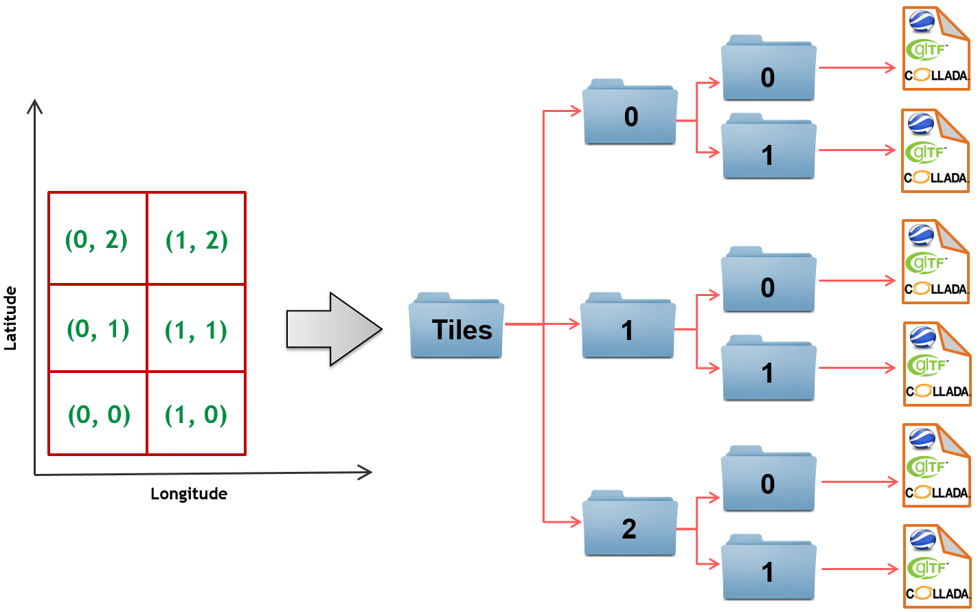
Fig. 4.75 Example: hierarchical directory structure for export of 3x2 tiles
Note
The Tiles hierarchy is also created if tiling is disabled.
In this case, a single visualization dataset is created per display form
and is stored at (0, 0) in the tree.
Export preferences
More fine-grained preference settings affecting the visualization export operation are available on the Preferences tab of the operations window [5]. Make sure to check these settings before starting the export process. A full documentation of the export preferences is provided in Section 4.6.7. The following table provides a summary overview.
Preference name
|
Description
|
General options affecting the visualization export as well as COLLADA/glTF specific settings.
|
|
Defines the styling to be used for the different top-level features.
|
|
Defines KML-based information balloons to be displayed when clicking on a top-level feature.
|
|
Controls elevation settings like the altitude mode and height offset for features.
|
Starting the export process
Once all settings are complete, the visualization export is triggered with the Export button [4] at the bottom of the dialog (cf. Fig. 4.73). If a database connection has not been established manually beforehand, the currently selected entry on the Database tab is used to connect to the 3D City Database. The separate steps of the export process as well as all errors and warnings that might occur during the export are reported to the console window. The overall progress is shown in a separate status window. This status window also offers a Cancel button to abort the export process at any time.
Output files
The export process will create several output files inside the export directory [1]:
- The main KML file as specified in [1]. This file links all visualization datasets as described above. For most viewers it should therefore be sufficient to just open this file in order to load and visualize the entire scene.
- The
Tilesfolder containing the tile files as described above. Note that every tile file might reference additional external files such as COLLADA/glTF files or texture images, which are stored relative to the location of the tile file. - One master JSON file per display form that contains metadata about the exported content. The name of the display form is added to the filename to be able to relate the metadata with a display form.
The following snippet shows the content of an example master JSON file. The JSON properties reflect the most relevant export settings.
{
   "version": "1.0.0",
   "layername": "NYC_Buildings",
   "fileextension": ".kmz",
   "displayform": "extruded",
   "minLodPixels": 140,
   "maxLodPixels": -1,
   "colnum": 29,
   "rownum": 23,
   "bbox": {
      "xmin": -74.0209007,
      "xmax": -73.9707756,
      "ymin": 40.6996416,
      "ymax": 40.7295678
   }
}
Applications can derive more information based on the provided metadata. For example, the length and width (in WGS84) of each tile can be determined using the following formulas:
Based on these values, applications are also able to use the following formulas to easily retrieve the row and column index of the tile in which a given point lies:
where X and Y denote the WGS84 coordinates of the given point.
For a bounding box interactively drawn in the scene, all intersecting tiles can also easily be identified. First, the row and column indexes for the lower left and upper right corner points of the bounding box have to calculated as shown above. Assume that the result is given as (R1, C1) and (R2, C2) respectively. A tile intersects with this bounding box if its RowIndex and ColumnIndex fulfills the following condition: