4.6.7.1. General¶

The General preferences dialog offers both common and output format-specific settings affecting the visualization export.

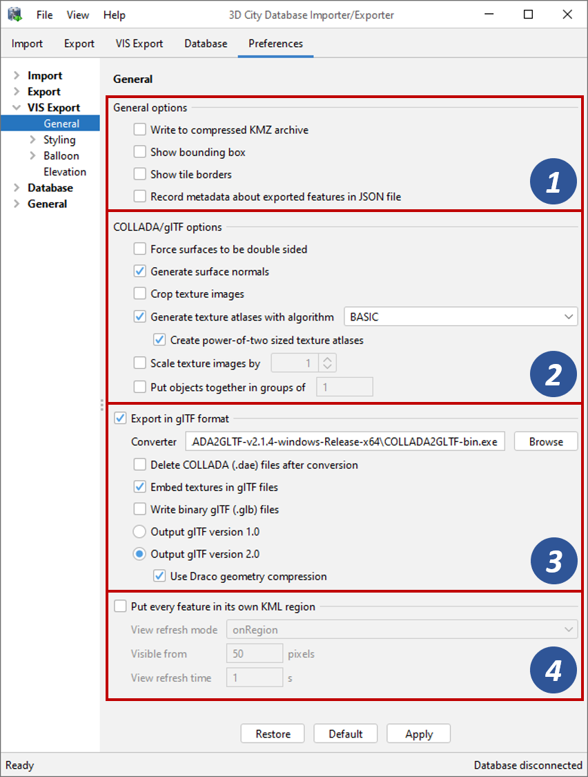
../../_images/impexp_kml_export_preferences_general_fig.png

Fig. 4.60 Visualization export preferences – General settings.

General options

By default, the export process creates one KML file per display form and tile in the Tiles output folder (see Section 4.6). When tiling is disabled, a single KML file is created for each display form instead. The file will either contain KML representations of the exported top-level features in case of KML-specific display forms, or references to COLLADA models in case of the COLLADA/glTF display form (also see Table 4.25). The COLLADA models will be stored in subfolders relative to the KML file. When choosing the option Write to compressed KMZ archive [1], all files per tile and display form are packaged into a single KMZ archive instead. This reduces both the overall size of the exported data and the number of output files and, thus, helps to minimize loading times when sending the visualization data over a network.

Note

The main KML output file specified on the VIS Export tab linking all files in the Tiles output folder (see Section 4.6) is always exported as uncompressed KML file independent of this setting.

Note

The KMZ archive format is only defined for COLLADA models and does not support glTF models. For this reason, the options Write to compressed KMZ archive and the Export in glTF format [2] are mutually exclusive.

With the Show bounding box and Show tile borders options [1], a user can specify whether the bounding box of a) the entire export area and/or b) each individual tile should be displayed in the viewer. If enabled, a separate KML geometry for each bounding box will be contained in the output files.

The Record metadata about exported features in JSON file option [1] lets you create an additional JSON metadata file in the export directory. This file contains the identifier, the envelope (as 2D bounding box in WGS 84) and the tile (as row and column index) of every top-level feature in the visualization export. The JSON file will have the same base name as the main output file specified on the VIS Export tab (see Section 4.6). The following snippet exemplifies the contents of the JSON file.

{
   "BLDG_0003000b0013fe1f": {
      "envelope": [13.411962, 52.51966, 13.41277, 52.520091],
      "tile": [1, 1]
   },
   "BLDG_00030009007f8007": {
      "envelope": [13.406815, 52.51559, 13.40714, 52.51578],
      "tile": [0, 0]
   }
}

This metadata is helpful, for instance, in case a viewer or application dynamically loads and unloads tiles and therefore has always just access to the features on tiles that are loaded. The metadata file can be used as index over all exported features in order to quickly find and access features even if their corresponding tile is not loaded.

Note

Make sure to enable Cross-Origin Resource Sharing (CORS) headers if you want to access the metadata file from a web client using a cross-domain request. CORS headers are additional HTTP headers in the response that allow the web client to access the requested data. This must be enabled on the server that hosts the metadata file.

COLLADA/glTF options

The COLLADA/glTF options [2] only apply to visualization exports in COLLADA and glTF format, which are triggered by choosing the COLLADA/glTF display form on the VIS Export tab.

A viewer typically checks for each polygon of a 3D object whether it is “visible” based on its face orientation. If not visible, the polygon is skipped from the rendering process (so-called backface culling) to reduce the number of polygons that have to be drawn and, thus, to increase the visualization performance. If your data contains polygons with a wrong orientation, they will therefore not be shown in the viewer. To disable backface culling and force the viewer to render all polygons, enable the Force surfaces to be double sided option (default: disabled). Be aware that this might decrease the visualization performance though.

The option Generate surface normals calculates the surface normal for each polygon and stores it in the visualization model (default: enabled). Surface normals play a central role in shading and for the amount of light the polygon reflects in a 3D visualization. The following Fig. 4.61 shows a building model visualized with (left) and without surface normals (right). When exporting textured models, surface normals often do not increase the visual quality. The option may be disabled in this case to reduce the output file size.

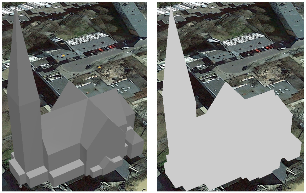
../../_images/impexp_kml_export_surface_normal_comparison_fig.png

Fig. 4.61 Different shadings of the same 3D object with (left) and without surface normals (right).

When working with textured models, texture images are sometimes larger than required for texturing the polygon. Loading massive texture data into a viewer may impact the visualization performance, so you should especially avoid loading unnecessary texture data. For this purpose, the Crop texture images option lets you cut the texture images for each polygon to the minimum required size during export.

Another option to optimize the visualization performance for textured models is to generate texture atlases (default: enabled). Instead of exporting one texture image file per surface to be textured, a texture atlas groups multiple texture images into a single file. This reduces the number of texture image files that have to be sent over the network and loaded by the viewer. The export operation will always create one or more texture atlases per top-level feature, but the same atlas is never shared between different top-level features. The texture atlases can be enforced to be power-of-two sized (default: enabled), which might be required for a viewer to efficiently manage the texture images.

In general, creating a texture atlas for a set of texture images is a combinatorial problem, also known as ‘knapsack problem’ (see [CGJT1980]). Different algorithms have been proposed in literature that differ in speed and packing efficiency. The export operation offers three different algorithms that can be selected in the preferences dialog:

BASIC: This algorithm recursively divides the texture atlas into empty and filled regions (see http://www.blackpawn.com/texts/lightmaps/default.html). The first item is placed in the top left corner. The remaining empty region is split into two rectangles along the sides of the item. The next item is inserted into one of the free rectangles and the remaining empty space is split again. Doing this in a recursive way builds a binary tree representing the texture atlas. When adding an item, there is no information of the sizes of the items that are going to be packed after this one. This keeps the algorithm simple and fast. The items may be rotated when being inserted into the texture atlas.
TPIM: The touching perimeter algorithm (TPIM, see [LoMV1999] and [LoMM2002]) sorts images according to non-increasing area and orients them horizontally. One item is packed at a time. The first item packed is always placed in the bottom-left corner. Each following item is packed with its lower edge touching either the bottom of the atlas or the top edge of another item, and with its left edge touching either the left edge of the atlas or the right edge of another item. The choice of the packing position is done by evaluating a score, defined as the percentage of the item perimeter which touches the atlas borders and other items already packed. For each new item, the score is evaluated twice, for the two item orientations, and the highest value is selected.
TPIM w/o image rotation: Same as TPIM but the rotation of images is not allowed when packing. The score is, thus, evaluated only once since only one orientation is possible. This variant is faster but less efficient compared to TPIM.

From these algorithms, BASIC is the fastest (shortest generation time) and produces good results, whereas TPIM is the most efficient (highest ratio of used area of the total atlas size) but also the slowest.

Caution

If you already imported texture atlases into the 3DCityDB, they can, of course, be used “as is” for the visualization export. Simply deactivate both the Crop texture images and the Generate texture atlases in this case. However, if the original texture atlases were created such that they are shared by more than one top-level feature, they will be exported redundantly for each top-level features and a viewer has to load the same texture atlas multiple times. To avoid this, it is recommended to both crop the original texture atlases and let the exporter generate new texture atlases from the cropped images.

To scale texture images is another means of reducing file size and increasing loading time. A scale factor between 0.2 and 0.5 often still offers a fairly good image quality while improving the visualization performance. The default value is 1.0, which means no scaling. This setting is independent from the generation of texture atlases and both can be combined.

Instead of exporting each top-level feature as individual COLLADA and/or glTF model, you can also choose to group multiple features into one model. Similar to texture atlases, this can help to reduce the number of individual models and files to be sent over the network and, thus, to improve loading times and visualization performance in the viewer.

Note

Only the first feature in a group is placed on the terrain model. All other features will receive local coordinates relative to this first feature. This might result in a wrong position on the earth surface if the features in a group are far away from each other.

Export in glTF format

In addition to COLLADA models, the Importer/Exporter can also export 3D contents from the database in glTF format. Technically, the top-level features are exported as COLLADA first and then converted to glTF using the open source COLLADA2glTF converter tool. There is a growing support for glTF models in various applications and especially in WebGL-enabled web engines and viewers.

Simply enable the Export in glTF format option to let the export operation create glTF models. This also makes additional glTF-specific settings available in the preferences dialog [3].

The mandatory COLLADA2glTF converter is available for Windows, Linux, and Mac OS X and is automatically installed with the Importer/Exporter. It can be found in the folder contribs/collada2gltf within the installation directory (see also Table 1.1). By default, this pre-installed converter is used by the export operation. You can choose to use another version of the COLLADA2glTF converter, in which case you have to provide the path to the executable in the Converter text field. Note that at least version 2.1 of the converter is required to be able to export both in glTF version 1.0 and 2.0.

By default, the glTF models are exported in addition to the COLLADA models. If the COLLADA models are not required in your subsequent processes though, they can be deleted after conversion by enabling the corresponding option to reduce the size of the overall export.

When exporting textured models, the texture images can either be exported as separate files relative to the glTF model (default) or be embedded in the glTF file. In the latter case, the base 64 encoded texture data is written to the glTF file. Both options have their pros and cons: if not embedded, viewers can first load and render the geometry and apply the texture images afterwards. This might result in a better user experience since content becomes visible quickly. On the other hand, all texture images have to be requested and loaded individually over the network, which might impair the overall visualization performance.

The exported glTF files can be further converted and compressed to binary glTF format. This can additionally help to increase loading and processing times.

The export operation supports both glTF version 1.0 and 2.0. The current version 2.0 of the glTF format is supported by most applications and tools and, thus, is used for the export by default. It also offers the possibility to compress the geometry data using the Google Draco compression technology, which significantly reduces the size of the output glTF files. For this reasons, the Draco compression is enabled by default but can be disabled by the user if required.

Put every feature in its an own KML region

With the Put every feature in its an own KML region option [4] enabled, an individual KML <Region> is created for each exported top-level feature. While the visible from settings on the VIS Export tab (see Section 4.6) only affect the visibility of each tile (or of the entire export area in case tiling is disabled), this options allows you to define additional and more fine-grained visibility settings that are applied to the KML <Region> element of each feature. The envelope of each top-level feature as stored in the database is used to define the spatial extent of this region.

When enabled, the Visible from parameter lets you control the visibility of each feature. The meaning of this parameter is identical to those on the VIS Export tab: When the feature is projected onto the screen in the viewer, it must occupy an area of the screen that is greater than the number of pixels specified here (in square pixels) in order to become visible. Note that this value is applied to all features the same.

The field View refresh mode specifies how the content of the KML <Region> is refreshed when the camera view changes. The following values are defined in KML and can be chosen in the preferences dialog:

Table 4.21 *Supported view refresh modes*¶
Refresh mode	Description
never	Ignore changes in the view.
onRequest	Refresh the content only when the user explicitly requests it.
onStop	Refresh the content n seconds after movement stops, where n is specified in the field View refresh time parameter.
onRegion (default)	Refresh the content when the `<Region>` becomes active.

As stated above, the parameter View refresh time specifies the number of seconds to wait after movement stops before the content of the KML <Region> is refreshed. This field is only active when the View refresh mode is set to onStop.

Note

The visibility settings per KML <Region> and top-level feature require that a viewer fully supports this KML mechanism (like, for example, Google Earth). The Cesium-based 3D web map client shipped with the 3D City Database (see Section 6) does not support this mechanism and, thus, silently ignore these settings.